Lab 3 - Perks of Being a Wallfollower

Wallfollower

Introduction

[Carolina]

The primary goal of this lab was to practice configuring, publishing and running code on our racecar. It is important for our team to become very comfortable with the process of setting up our robot hardware, as this is something we will repeat throughout the semester in every future lab. In this lab, we adapted previously-written code from Lab 2:Wall-Follower Simulation to enable our racecar to autonomously follow a wall at a certain distance. Adapting this code from a simulation to a real-world environment presented technical challenges. Finally, we implemented a safety controller that prevents our robot from incurring damage – a key element of a physical robot platform that was previously unnecessary in the simulation context. We took a unique approach to our wall follower by implementing a nested feedback loop controller, and then created an effective safety controller.

Technical Approach

Initial Set Up and Hardware Configuration

[Carolina]

The initial portion of this lab involved configuring our robot’s hardware and connecting it to the router, which allows us to publish code to the robot. At first, the car would not connect to our router, but after physically connecting the car to a monitor, keyboard and mouse, we were able to visualize its settings and enable automatic sign in to avoid this issue in the future.

We then tested several hardware components located on or linked to our robot. First, we ensured that we could control our robot manually with the joystick – this is important to be able to override our autonomous code in case of unexpected errors, or to be able to control the robot for testing programs that don’t automate its movement. We ran test files and also demoed the joystick on our own.

Once we ensured the joystick was functioning, we moved on to testing our car’s IMU. Although we haven’t used the IMU yet during a lab, we know that the features of the IMU (the gyroscope and accelerometer) will be useful in the future to allow our robot to perform dead reckoning.

Finally, we tested the lidar sensor. The lidar acts as the eyes of our robot and allows it to perceive objects through laser scanning that sends the robot the distances of a series of points in its vision. We need lidar data to be able to detect walls and other objects for future labs. To test the lidar scanner, we visualized the lidar data using RVIZ (running roscore on our robot). We then put our hands in front of the robot and watched how the data points on RVIZ responded. We also ran our wall follower code and visualized the lidar data, as shown in Figure 2.1.1. Below.

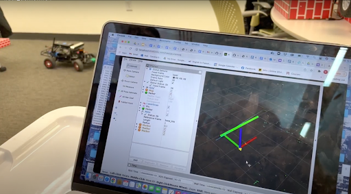
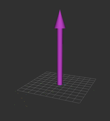
Figure 2.1.1. RVIZ visualization of lidar data (left) and IMU (right)

Wall Follower Implementation

[Vedang Lad, Quinn Bowers]

The car uses negative feedback to maintain its distance to the wall. The car first uses lidar to detect its relative position to the wall. A controller then reads the $error$, or the difference between desired distance ($d_r$), and actual distance ($d$), and outputs a new steering angle for the car.

The car’s lidar detector produces a list of 2D points. Processing these to produce an estimation of wall location can be sensitive to outliers. To detect the wall, we run a linear regression on a subset of the points, selected based on which side we expect the wall to be on. Weighting the points by $\frac{1}{r^3}$ allows the regression to treat closer points as more "important" than distant ones. This weighting scheme has two main benefits. Firstly, the linear regression passively rejects outliers. The lidar module sometimes returns a distance of max_distance instead of the actual distance to an object at the reported angle. These points are given negligible weight, and so will not throw off the wall detection. The other benefit of this weighting scheme is how it responds to corners. Decreasing the weight of distant points allows the robot to look straight ahead. Points that are far away and far from the wall will also not throw off the wall detection. Once the robot is close enough to the corner that it should begin turning, the points straight ahead will have enough weight to change the wall detection, causing the robot to begin to turn.

There are two key ingredients that make our wall follower implementation different from other groups. The first is the use of two nested proportional gain controllers, which allows for greater wall tracking abilities. This is particularly useful in situations where the racecar can lose the wall, such as wall protrusions and hidden corners. While one controller tracks the angle the other controller tracks the wall distance. This unique nested structure prevents overcorrection errors that can be seen in a standard PID controller.

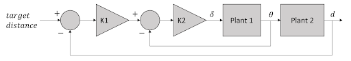
Figure 2 Block Diagram of the wall follower feedback loop. The inner feedback loop controls the angle of the car with respect to the wall, $theta$. The outer feedback loop controls the distance of the car with respect to the wall.

Safety Controller Implementation

[Ishita Goluguri]

The safety controller is a program that runs on the robot alongside all other programs. Its purpose is to prevent the robot from crashing into sudden obstacles, whether it is a person walking into its path or another robot. However, the safety controller cannot be restrictive and prevent the robot from its actual functionality, which in this lab, was to follow the wall.

As an overview, the Safety Controller takes the current path of the robot and uses this to predict the robot’s trajectory over a certain brake time, which is currently set to be 0.5 seconds. If there are obstacles detected within a minimum safe distance from the trajectory, which is currently 0.5 meters, then the robot stops immediately.

The safety controller utilizes one publisher and two subscribers. The publisher, ackermann_publisher, publishes messages of the type AckermannDriveStamped to the topic /vesc/low_level/ackermann_cmd_mux/input/safety. As seen in Figure 2.4.1, these messages get the second highest priority, with only the joystick getting higher priority. The safety controller also takes precedence over the AckermannDriveStamped messages published to the navigation topics: "/vesc/low_level/ackermann_cmd_mux/input/nav_i." The two subscribers, drive_subscriber and lidar_subscriber subscribe to the topics /vesc/low_level/ackermann_cmd_mux/output and /scan respectively. The drive_subscriber retrieves the AckermannDriveStamped messages navigating the car at any given time, and the lidar_subscriber retrieves information about objects around the robot through lidar data.

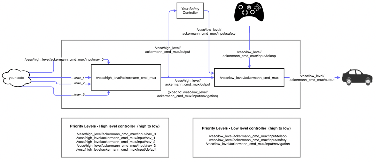
Figure 2.4.1 Slide from 6.141 lecture

The drive_subscriber calls the function drive_callback, which sets the car’s speed and angle to the current values in the class variables. The lidar_subscriber calls the function lidar_callback, which analyzes the LiDAR data to determine if the robot should halt.

The function lidar_callback begins by creating a point array, which contains the x and y coordinates of the lidar points with respect to the robot as the origin:

safety_controller/src/safety_controller.py

points = [( r*np.cos(theta) + 0.3, r*np.sin(theta), r, theta) for r, theta in zip(data.ranges, angles)]

This function takes the data.ranges values, which are passed in as a series of angles with corresponding distances, and converts it to cartesian coordinates The x-coordinate was increased by 0.3 to translate the points from coordinates with respect to the lidar frame to point with respect to the robot frame.

Next, the curvature is calculated from the car’s current steering angle by taking the reciprocal of the radius. $K = \frac{1}{R} = \frac{sin(steering\_angle)}{L}$, where L and steering_angle are as shown in the diagram. We chose to use the curvature rather than the radius, because the radius can approach infinity and thus has no limit, but the curvature approaches 0. Next, the look-ahead distance is computed by multiplying break_time, velocity, and the safety_factor. These factors were chosen because they took into account the amount of distance the robot was predicted to move before it could stop (break_time*velocity), and also a little bit of extra distance for safety purposes, which is added through the safety_factor. In addition, there is a minimum_safe_distance that points must be away from the robot’s trajectory to account for the width of the robot and any error.

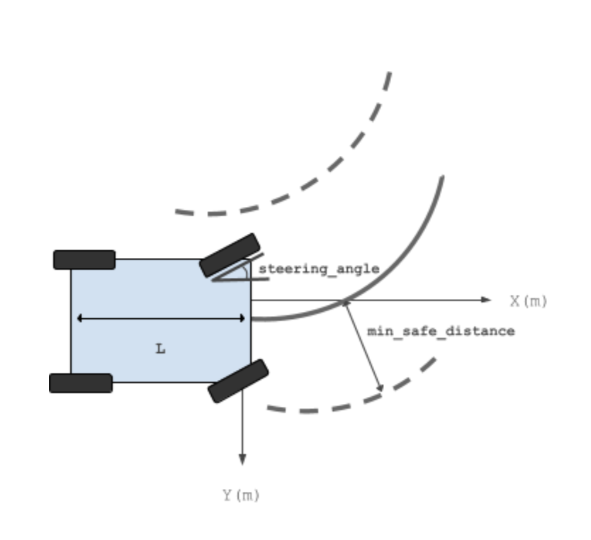
Figure 2.4.2 Diagram describing variables in trajectory prediction. $L$ is the length of the car and remaining parts are as labeled.

Next, we check if there are any points that fall in the danger zone described above. We also throw out any points that are too close to the LiDAR, which are the sensor detecting the robot itself, and any points with angles less than $\frac{\pi}{2}$ or greater than $\frac{\pi}{2}$. This prevents the robot from sensing points behind itself.

The points from the LiDAR are converted back into polar coordinates with respect to the robot’s center of origin, and checked to see if they are in the problematic region. It’s important to note that the robot’s center of rotation is not the same as the center of the robot, but is needed to determine whether the points fall in its trajectory, thus necessitating the switch from the given data to cartesian coordinates and then back to polar coordinates.

If the points are within the danger zone, they are appended to the danger array. If the danger array is nonempty after scanning through all the allowed LiDAR points, a stop command is sent through the method send_stop_message(). The method publishes a drive message with speed 0 and angle 0 using ackermann_publisher. This stop command takes precedence over the navigation commands and stops the robot immediately. In the case that no danger points are detected, no stop command is sent, and the robot navigates normally.

Figure 2.4.3 Video demo of the car following the wall via the wall follower code, and reacting to an unexpected object in the path via safety controller commands

Experimental Evaluation

Experimental Procedure, Parameters and Purpose

[Quinn Bowers]

To evaluate the effectiveness of our wall follower, we measured its response to a step input, both in reality and in simulation. To create a step response, the robot was driven along a wall that jutted suddenly outwards, as shown in figure 3.1.1. This wall was assembled with cardboard boxes in reality, and was drawn manually in simulation.

The step response of the car was then analyzed. Because we do not currently have a reliable method of determining the car’s location in space available to us, we instead examined the error signal over time. The step response can be analyzed to determine the peak error and the time it takes for the car to settle back into equilibrium, $t_s$. Our design goal is to minimize these values as much as possible; a high peak error means that the car may be too far away from the wall, or too close. If the error ever exceeds the target distance, this implies the car has crashed. A large settling time often implies that the car is oscillating for a long time, causing it to waste motion. A high peak error is unsafe. A high settling time is wasteful. The analysis in the following sections shows that our controller has very acceptable error and settling time at low speeds, but can sometimes fail at high speeds.

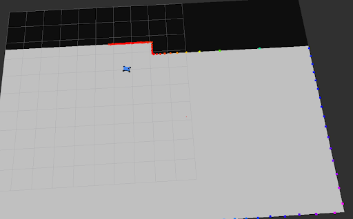
Figure 3.1.1 The robot navigating a custom simulation. We used a custom map to determine the robot’s response to stimuli in a variety of different target distances and speeds.

Simulated Robot Evaluation

Figures 3.2.1-3 depict the step responses of the simulated robot. Each figure shows the response of the robot at different target distances, but the same speed. From the figures, it can be observed that both maximum error and settling time increase with target distance. It is interesting to note that maximum error does not seem to increase with speed. Settling time decreases with speed, which matches the fact that the car is moving faster and able to adapt more quickly.

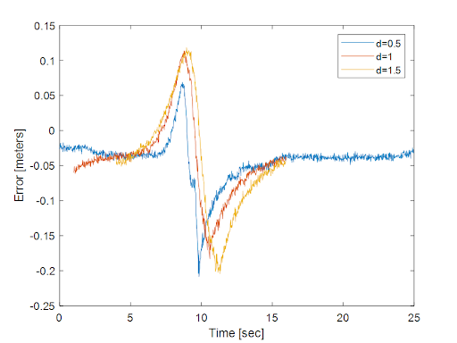
Fig 3.2.1 Step response of the simulation car with different target distances. All cars are traveling at 0.5m/s.

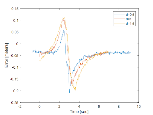
Fig 3.2.2 Step response of the simulation car with different target distances. All cars are traveling at 1m/s.

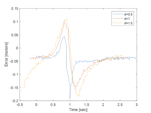
Fig 3.2.3 Step response of the simulation car with different target distances. All cars are traveling at 3m/s.

Physical-robot evaluation

Evaluating the physical robot was not nearly as smooth. The car suffered a number of technical difficulties that took some time to resolve, reducing the amount of analysis we could do. Additionally, real-world data is seldom as clear as simulated data. Figure 3.3.3 shows an experimental step response of the car. The time steps between data points are noticeably less uniform than simulation data, and the error reading is noisier. Figure 3.3.4 shows another step response with even more noise. The real-world data was sufficiently noisy and inconsistent that it could not be analyzed the same way the simulation data was. Indeed, much of our real-world data had to be completely thrown out.

Nonetheless, there are still conclusions to be drawn from our experiments. Figure 3.3.5 shows a step response where the car oscillates. This behavior is also shown in Figure 3.2.1. No oscillation was observed in the simulation. This implies a mismatch between the car in reality and the car we modeled. This mismatch is to be expected, however we did not anticipate the dynamics of the hardware car to be different enough to cause semi-stability in our controller.

We can also notice that in many cases, the car responds quite well to step responses. Figure 3.3.3 shows a characteristic step response of the car traveling at low speeds. The peak error is only 0.25 meters, and the settling time is roughly one second.

Finally, we note that the car behaves more stably at a greater distance from the wall. Figures 3.3.5 and 3.3.4 depict step responses of the car moving at the same speed, however the car is 1.5 meters from the wall in figure 3.3.4 and only 1 meter from the wall in figure 3.3.5. When further away, the response is still messy, but does not feature the same large oscillations as in the near case.

Figure 3.2.1 The hardware car following the wall. The inner loop gain has not yet been adjusted. The car oscillates semi-stably as it follows the wall.

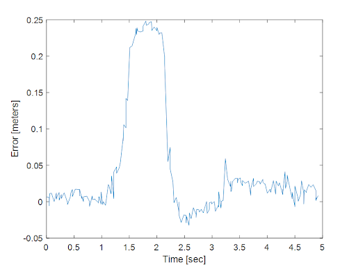
Figure 3.3.3 Step response of the hardware car. Target distance is 0.5m, and car velocity is 0.5m/s.

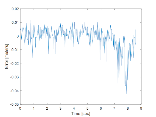
Figure 3.3.4 Step response of the hardware car. Target distance is 1.5 meters, and car velocity is 3m/s.

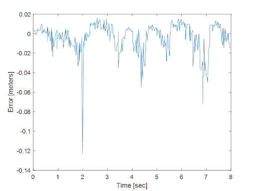
Figure 3.3.5 hardware step response. Target distance is 1m, and car velocity is 3m/s. The car oscillates noticeably after the step response, and is in fact only semi-stable. These oscillations do not decay with time.

Conclusion

[Vedang Lad]

In this design phase, we constructed an essential framework for success. Just like a human, for a robot to successfully interact with its environment, it must learn to navigate it safely. We achieve this by implementing an accurate wall-following mechanism that ensures collision-free motion regardless of the shape of the wall. Unlike other PID controllers, our group’s controller is unique in that it nests two proportional controllers, not one. This mechanism prevents losing the walls on turns since the outer controller can correct errors of the inner controller. An onboard safety controller brings the robot to a smooth stop in the event of a collision, which is a similar feature to life-saving auto-brake mechanisms that have become a standard feature on cars today.

Due to our robust simulator code, we can seamlessly transition from a simulated robot to one in the real world. We test the robot in three different environments to ensure its success. The first is on an elevated box, which confirms successful wall detection and eliminates the possibility of collision. The second environment is a classroom wall, which tests for wall following in an obstacle-free environment. The third and most challenging test is in the basement of Stata. While also testing the safety controller, the group ensures the robot’s success is not environment-specific.

Rigorous testing and problem solving would be impossible without collaboration and resourcefulness. For instance, when faced with connectivity issues, the group found a nearby TV, mouse, and keyboard to find a solution. If challenged by an unsolved bug, all group members pause their respective work and attack the problem together. When stuck, the group asks for guidance on how to solve the issue at hand. For instance, when “phantom” lidar points appeared on the robot and rigorous troubleshooting did not find a solution, reaching out to the TA enabled the group to reach the solution.

Overall, the group completed the lab, creating a seamless transition to the next lab. We are excited to take on a new problem after this lab. More importantly, we look forward to continuing our pursuit of cultivating strong technical and interpersonal skills. By introducing a vision system, we will be able to navigate now with eyes allowing the robot to make smarter decisions in the environment. Instead of following a wall, the robot will follow a line that requires higher precision in movements. Furthermore, it will learn to stop in the presence of a cone. While more information means higher complexity, the group is ready to tackle this next challenge with the same drive as we did the first.

Lessons Learned

Vedang Lad Time management was the essential ingredient that I learned from this lab. Having taken advanced physics and mathematics classes, I had a strong understanding of the principles of PID controllers; however, I did not anticipate the time taken to design, test, and implement my own. Luckily, with the help of all my group members, we completed all of our assignments promptly. A key lesson I learned in collaboration was that more is not always better. When each group member found a different role to fill, we were far more productive and had a much clearer direction instead of everyone working on one assignment. We divided up the work to ensure that we were efficient with our time. A key lesson in communication that I learned was not to be ashamed to ask for help. After spending an hour trying to figure out why mysterious points were appearing on the lidar sensor around our robot, I reached out to a TA for help. It turned out that that robot was detecting itself on the lidar, a common issue. At that moment, I realized the importance of struggling with a problem and recognizing when to reach out for help. I hope to build on the ever-growing skill set as we continue work on the labs.

Ishita G A key skill I learned during this lab was splitting work up efficiently. A strategy I’ve used in past group work is to take the same work and split it up evenly among the different members of the group. However, in this lab, we split it up according to our various strengths, and as a result, we got it done much faster than we would have otherwise. In addition, we ran into many challenges. Sometimes, there was no viable explanation other than that it simply does not work. While momentary frustration is expected and understandable, it was important for us to progress past that feeling and think together about how to improve together. In addition, our team learned a lot about the resources available to us as a result of the challenges we faced. We initially tried to figure everything out by ourselves, but after we realized it wasn’t working, we branched out to asking other classmates, asking on Piazza, and asking a TA during office hours. Many of our issues were solved through a combination of all three of these methods. Working on this lab and going through the initial setup taught me many strategies that I can continue to use throughout this class and beyond.

Carolina W Perseverance despite frustration was a key skill learned during this lab. Our team faced a number of challenges, from missing Ethernet cables, problematic router connections, and unusual IMU errors to hidden bugs in our code. We practiced resourcefulness, collaborating as a team to locate replacement hardware from wherever we could find it – borrowing cables from friends in our dorms and using the TVs in lounges as monitors. Being resourceful helped us to bypass these issues and continue to make progress on the lab without becoming stuck. Additionally, we found it was complicated at first to communicate when there were so many different elements of the lab that needed to be addressed – however, we found that using a messenger chat to stay up-to-date with one another was an effective strategy. I personally became very comfortable with the setup process involved in using the robot – what hardware needs to be connected and what commands need to be run in terminal before we can start pushing code to the robot. I also learned how to use RVIZ effectively to visualize Lidar and IMU data, which will be very useful as we pursue future labs.

Quinn Bowers One of the biggest lessons I learned over the course of this lab was the necessity of taking clear, copious notes. I frequently found myself looking up the same linux commands. This was not too much of a challenge or use of time, but the same lesson applied to debugging; After spending multiple hours fixing the robot’s connection to the joystick, I forgot a small, crucial detail and spent another several hours debugging the same issues. Having these lessons written down will help not only myself, but also democratize our progress to avoid one person knowing all the tips and tricks. Another important lesson is to keep organizational frameworks as consistent as possible. We switched up our github repository structure twice (once to a new layout, then back when the TA’s told us this was a bad idea), and while this did not take too much time, the back and forth made it tricky to keep everyone up-to-date on how to stay organized. As a final note, I need to get better at figuring out when to pass off my knowledge and hand off tasks to others, or to just buckle down and hammer them out. I have a reasonable degree of linux experience, and often found myself scrambling to get things set up and running so others could get to work. I also have a tendency to underestimate how long tasks will take to complete. It is likely that I should be teaching these tasks to other people, to decrease my personal workload and also ensure the team is equally functional without me.

Presentation

Download Links

Briefing Slides: Download Slides

Report: Download Report