Lab 6 - Pure Pursuit of Happyness

Path Planning

Introduction

[Carolina]

This lab built off of our previous accomplishments in the localization lab to implement a powerful ability on our robot – navigation. Navigating our robot in an environment involves finding a path to take through the environment and then successfully following this path to reach a goal destination. To accomplish this path-planning, we implemented two path-finding algorithms, $A*$ and $RRT*$, and then used the pure pursuit method for following the generated paths. Integrating the two to give our robot the capacity to create and execute paths was as simple as running both of the algorithms simultaneously. We evaluated each algorithm in simulation and then tested the combination of the algorithms on hardware, finding that our robot was able to successfully generate paths and reach a goal node in a reasonable amount of time. We found that there is room for tuning in our code, as well as a need to further refine our localization code from the previous lab to work better with pure pursuit. However, our navigation approach was overall successful, and will be greatly helpful to us in the final challenge as our robot learns to drive safely in a unique “city” environment.

Technical Implementation

A*

[Ishita]

Moving a robot between two points in space is a daunting task. One of the ways we approached this problem was by adapting an algorithm we’d heard of in previous classes: $A*$. $A*$ is a graph algorithm that finds a path between two points, and optimizes the path to minimize its length. To discretize a map and turn it into a graph, we used each pixel on the map as a node as shown in Figure 1, and considered there to be edges between each node and its four neighbors. For a given point $(x,y)$ in pixel coordinates, the four neighbors were the elements of ${(x-1,y), (x+1,y), (x,y-1), (x,y+1) }$ that were within the map’s bounds. The decision to not include diagonal neighbors was made to reduce computation time, and because the difference in distance between a diagonal map and one that stepped one edge in each direction was small enough to be negligible.

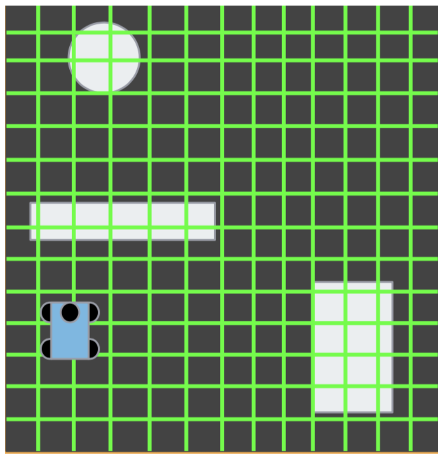
Figure 1: This diagram shows the discretization of a map into pixel squares.

Our implementation keeps track of the minimum distance between the start node and every other node in a dictionary, and updates the dictionary every time a shorter path is found between the two nodes. The algorithm generates the four neighbors of the current node and adds the ones that have not yet been visited to an open set. It then treats this set as a priority queue, and uses a heuristic to determine which should be chosen next. The heuristic sums the distance between the node and its current neighbor with the linear distance between the neighbor and the goal to optimally pick which neighbors should be explored next. This heuristic was used over alternatives such as Dubins curves because experimentation showed that linear distance worked better with discretization. After this, the node is added to a visited set to ensure that it is not revisited. In this manner, each node is visited exactly once, reducing computation time. When the algorithm chose a path that reached the goal node, this was chosen as the optimal path since the algorithm had already been optimizing at every step.

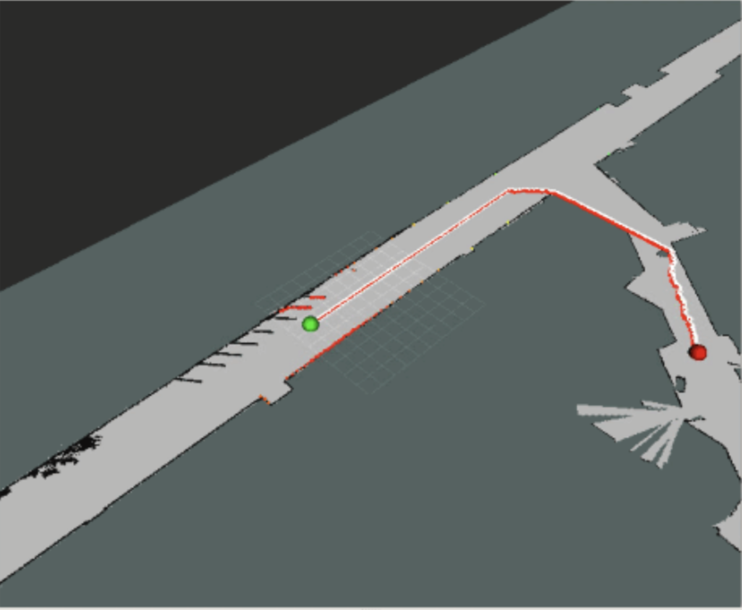
Figure 2: Sample $A*$ map between two points

In practice, the $A*$ maps chosen sometimes contained very small line segments as shown in figure 2, which would make it difficult for the car to actually follow the paths. Some of these issues were addressed with creative manipulations of the map. We found that dilating the map made the robot less likely to crash into walls by giving it a margin. In addition, we eroded the map to rid it of extraneous points before converting the map into a graph and running the algorithm on it.

RRT

[Tiffany]

An alternate type of path planning algorithm is a sampling based algorithm, which randomly chooses points in the map to pass through and then checks for collisions, speeding up the process by avoiding the need to generate and search through a graph of the entire map.

We chose to implement $RRT*$ as our sampling based algorithm. Our implementation had several iterations as we optimized the code. At first, we started with a simple $RRT$ implementation: generating a random point, generating a path between that and the nearest point already in the graph, seeing if that path reaches the end, and if not, continuing to generate the tree. While this method was fast, as it stopped as soon as a path to the end was found, it also allowed for non-optimal paths. To improve this, we created what we called $RRT+$, which continued generating paths until we had sampled a given number of points, stored the distances of all the paths that made it to the end and chose the best from among those. Finally, we implemented $RRT*$ which updated the paths as it generated points by trying to “steal” the shortest path of previous nodes located within a box centered at the new node. This created much more optimal paths, but at the cost of speed.

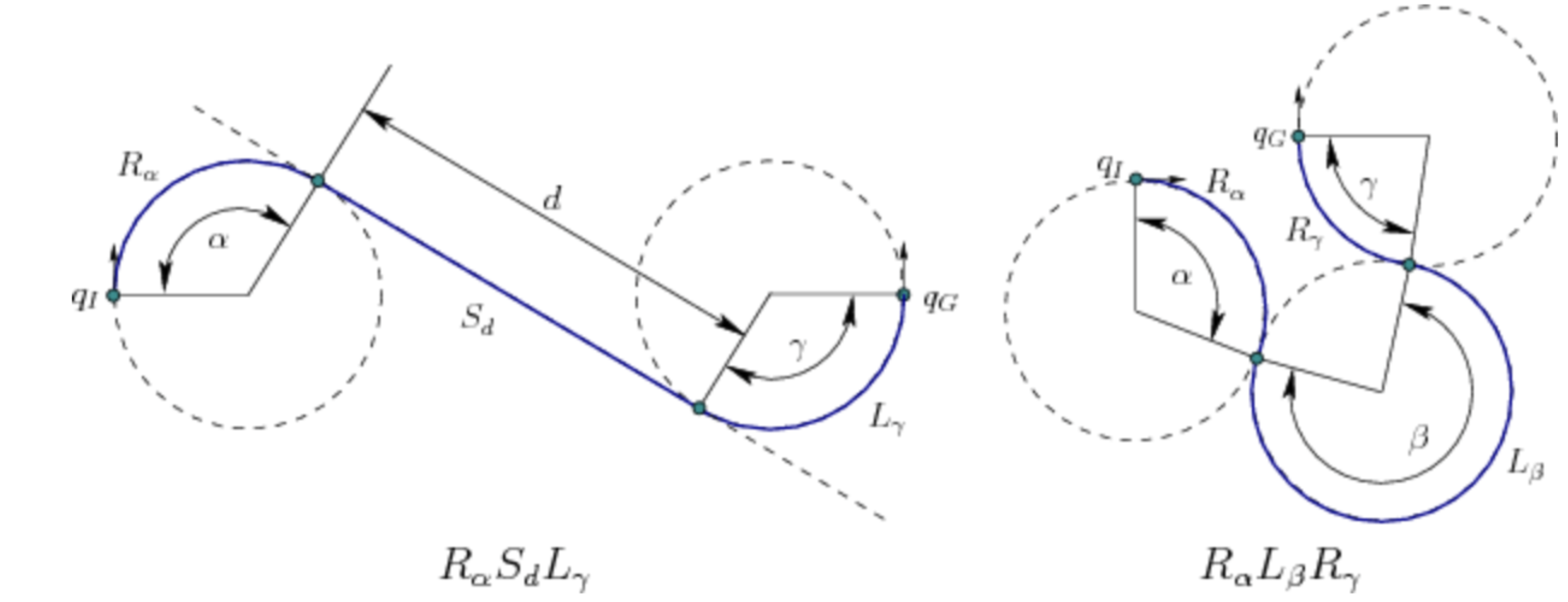
Figure 3: Examples of possible Dubins curves which guarantee optimal possible paths

By changing the cost metric for distance to Dubins curves, we improved the results of our path planning algorithm. Dubins curves allow us to find the optimal path for a forward-only car by saying that the shortest path for such a car is some 3-turn combination of 3 possible directions: Left, Right, and Straight. In order to create smooth curves which were possible given the robot’s current position and robot’s movement capabilities, we used these as our cost metric in the $RRT$ implementation. This made the path smoother and only represented paths that the car could actually take which was beneficial for pure pursuit.

Comparing Search and Sample Algorithms

We chose to use the $RRT$ algorithm as it was faster than $A*$ and implemented Dubins curves as the cost function, making it more practical to test with and creating only possible paths. By using Dubins curves as the cost function, the path-planning algorithm was able to incorporate the dynamics of the car and generate only paths the car would possibly be able to take. $RRT$ works faster, in O(nlogn), by avoiding the need to create a graph of the entire space and then subsequently search for it as $A*$ must, taking O($4^n$) time. In this sense, $RRT$ is better for large spaces like the Stata basement which would be expensive to do with $A*$. Our $RRT$ implementation avoids the need to search once the tree is created by storing parent pointers, speeding up the implementation. While $A*$ generates optimal paths, $RRT*$ generates optimal paths as the number of samples approaches infinity. In this case, when we strongly limit the number of samples, $A*$ created more optimal paths than $RRT$. As the number of samples increases, however, $RRT$ becomes increasingly optimal while not taking too long to run. As a result, $RRT's$ benefits outweighed the potential drawbacks of having potentially less optimal paths.

Pure Pursuit

[Vedang]

The pure pursuit portion of the code combines all of the components of this project. Our pure pursuit implementation is similar to that implemented in Lab 4: a simple two step algorithm that repeats indefinitely. The first step is to determine a point to drive to and the second step is to simply drive to the point.

Pure Pursuit: Determining the Point

Given a discrete trajectory, determining the point to drive to is the most challenging of the two steps. To solve this problem, we form a circle around the car, the radius being the value self.lookahead. The first step of the algorithm is to drive to the closest segment that intersects the lookahead circle. This value is constantly calculated throughout the robot’s motion with the use of efficient numpy operations. We approximate line-segments with infinite lines, and calculate the shortest distance to the given line segmentation using the point to line vector formula. This is clearly outlined in the diagram below, where arrows are represented by trajectories formed by path planning algorithms, and the dotted line represents the shortest distance.

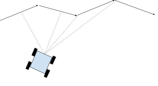
Figure 4: In Pure Pursuit, the first step is to calculate the distance to all of the segments, shown by the dotted line above.

Once we have picked a segment of interest, we need to find a point on the segment. This will become the segments that we will drive toward. This is calculated by solving a quadratic equation, by equating the equations of a line and a circle, which results in two solutions. We pick the solution that takes us forward on the trajectory. This math problem is generalized to the diagram that we see below.

Figure 5 In Pure Pursuit, the second step is to calculate the intersections of a segment on the self.lookahead circle, defined by the radius $r$ above. If the car were facing right, we would drive to the intersection closer to $p_2$

With creative freedoms in our implementation, we include a second “back-up” lookahead if the first one fails. This backup lookahead remains at the start of the closest segment that lies at a distance of 1.5*self.lookahead distance. This second lookahead point is essential for navigating dense trajectories, where the normal lookahead distance may fail. In the animation below, at the end of the trajectory, you can see that the first lookahead point, shown by the red dot, lies outside of the trajectory. The racecar can navigate to the correct finish point because it lies on the correct finish trajectory. This is how we determine the point, now we must just drive to it.

Pure Pursuit: Driving to the Point

This last part is arguably the easiest of all. Once we have determined a point to drive we must control the steering angle. If the absolute value of the steering angle lies outside of $0.25$ radians, we decrease the velocity of the racecar by a factor of 1-self.steering_angle. This ensures an accurate trajectory following a variety of turns. This information is best conveyed in the diagram below, which outlines the formula for the steering angle and how to drive to the point of interest.

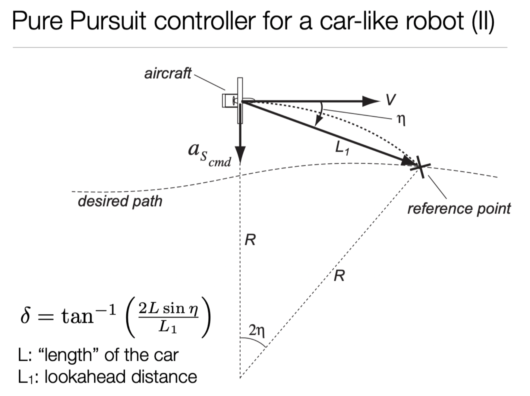
Figure 6: This figure shows how step 2 of pure pursuit works. Once a point is chosen, the steering angle is changed to the equation above in order to drive to the point.

Evaluation

$RRT*$ and $A*$ Evaluation

[Carolina]

To evaluate $RRT*$ in simulation, we looked at the overall distance of our path, the time it took to generate the path, and the smoothness of the path. Ideally, we would generate shorter, smoother paths in less time. Smoothness is especially important because in real life, we can travel a smooth path faster than a jagged path. Our car has to slow down to make sharp turns, but can take curves at a higher speed.

We facilitated the error-logging process in this lab by creating a simple error logging script with methods to write to a file. We called these methods in our code to record the full distance of the generated path, the time it took to generate (found by subtracting rospy.get_time() at the start of the path generation from the time at the end), and the full trajectory of the path, which we would evaluate later.

To run tests repeatedly using the same positions for both algorithms, we decided not to use RVIZ tools (giving it poses in the exact same position would not have been possible). Instead, we created a script based off of pose_init_pub.py, called destination_pub.py, which published a goal node directly to the robot. We first ran pose_init_pub with a position of $(0,0,0)$ to initialize the robot, and then used destination_pub.py to publish one of three positions in different locations on the Stata basement map (which were found previously using RVIZ tools). Publishing a position to the robot started the path-planning algorithm, and we repeated the trial for each position.

[Quinn]

$A*$ was evaluated the same way as $RRT$; we examined the length and curvature of the produced paths, as well as the time it took to compute them. The results are shown in Table 1 below.

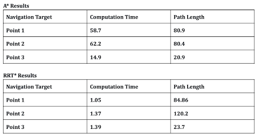
Table 1: Experimental results of two path planning algorithms. Both algorithms used the same set of points

We can see from the data some clear trends. Firstly, we notice that $RRT*$ runs in mostly constant time, regardless of the particular point it is navigating to. This makes sense in the context of the algorithm: $RRT*$ generates and processes a fixed number of points, so the process should take the same amount of time.

$A*$, on the other hand, has a significantly more variable runtime. With reasonable confidence, we can notice that runtime scales linearly with the final distance of the path. This also makes sense in the context of the algorithm; $A*$ exits as soon as it finds the optimal path to the destination point. Before then, the algorithm will have to search a number of points proportional to the path length, which will take a runtime proportional to the path length.

We now compare resultant path lengths; $A*$ produces shorter paths in every case. This is expected; $A*$ is guaranteed to produce optimal results for its cost function. $RRT*$, for comparison, is a random algorithm that does have guarantees on its runtime, but gives up its guarantees on path length. Furthermore, while not documented here, $RRT*$ will generate paths of different lengths every time it is run. It is not deterministic. In the cases above, $A*$ produced paths that were on average 10% shorter than $RRT*$.

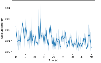
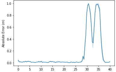
Pure Pursuit Evaluation

[Ishita]

The goal of pure pursuit was to help the robot follow the path that it received from the path planning algorithm. Thus, to evaluate this , we recorded the absolute error of the robot’s path (current position - intended position on the map). We recorded error as the robot ran three different paths, and also tested for three different speeds. For the most part, the error recorded is low, indicating that the pure pursuit worked well. However, we see large error occurring when the robot makes turns at high speeds, indicated by the spikes in the graph below. This error is caused by localization, because our robot goes off its predicted position, and the change is too fast for localization code to work well. After much experimentation, we’ve determined that it seems to be our localization code that is the issue. In addition, with the true odometry location, the plots should turn out similarly to what the low speed plots looked like. The three graphs from our resulting data are shown below.

0.5 m/s

1.0 m/s

2.0 m/s

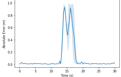
Figures 7,8,9: Graphs of pure pursuit error over time. Notice the significant jump in error when the car was turning. In addition, note that the y-axis for the first graph is much different than the other two.

Hardware Performance Evaluation

[Carolina ]

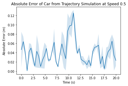
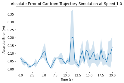
As a final step in this project, we evaluated the performance of our path-finding and path-following algorithms together on the physical robot. To integrate the code, we simply ran the launch files for $RRT*$ (since it showed better performance than $A*$ in simulation) and pure pursuit simultaneously, and published points to the robot using destination_pub.py. We ran the robot using the same goal node, but we changed the speed for each trial (0.5, 1 and 2 m/s). All of the types of error logged during the simulation trials for path-finding and path-following were logged during these trials as well – we recorded the total distance of each path, the time it took the robot to complete the path, and the absolute error over time.

0.5 m/s

1.0 m/s

2.0 m/s

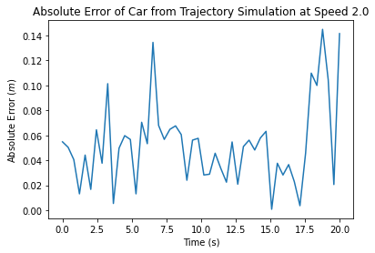
Figures 10,11,12: Graphs of the absolute error (car position - trajectory position) over time for trials at 0.5, 1.0 and 2.0 m/s. The first two plots also indicate a shaded error region, as multiple trials were conducted at these speeds.

Time and Path Length in Hardware Evaluation at Different Speeds

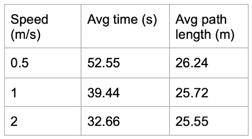
Looking at our absolute error plots, we can see that our robot’s error is fairly low at a speed of $0.5$m/s, ranging from $0-12$ cm with an average of about $6$ cm. However, as we increase the speed, our error increases, peaking at $14$cm and $35$cm at one point at a speed of $2$m/s. In terms of speed, we can see that our robot clearly runs similar-length paths slower at $0.5$ m/s – dividing the path distance by the run time yields about $0.499$ m/s. However, there is not a significant difference (only about 7 seconds) between the car running a path essentially the same length at $1$m/s and $2$m/s. If we look at the distance over time for both trials, we see the average speed of the car was $0.65$ m/s and $0.78$ m/s, which are $65$ and $39$ of the set speeds, respectively. This reduction in speed is due to the curvature of this path – in our pure pursuit code, we adjust our speed to handle turns safely, and so even with a higher given speed, there is a limit to how fast the robot can be at any point due to the curvature of our path. However, as established from individually evaluated pure pursuit and $RRT*$, there is room for improvement in both algorithms, as well as in our localization code, that would lead to a better combined result and would enable us to reach higher speeds.

Conclusion

[Quinn B ]

This lab represents the most complex combination of systems we have yet implemented. We first implemented two solutions to the problem of path planning. We found paths with a search based algorithm, $A*$, and a random sampling based algorithm, $RRT*$. Because of the significantly better runtime, we chose to use $RRT*$ for future path planning. Newly armed with both path planning and localization algorithms, we could now implement a pure pursuit controller, to drive the car along $RRT*’s$ generated path. When testing the combined system, we found that our path planning algorithms worked equally well in simulation and in hardware, but that our robot was less able to follow trajectories in hardware than in simulation. After much debugging, we narrowed down the culprit to our localization algorithm. This part of our software stack requires tuning or replacement in the future, before it can be used reliably in the final competition. Like our robot Dizzy, we look forward to the race!

Lessons Learned

Vedang L: A key lesson that I learned from this lab was the advantages of getting your code working early. Being in-charge of the pure pursuit implementation on this project, , I worked diligently to finish my code before the end of the weekend. Without essential explanations I received from the TAs at the start of the project, there is no way I would have a high level understanding of the project. This left me time to optimize my code and solve issues that arose when we tried to integrate the moving parts of this project. From this experience I learned how important it is to “own” your code. This means to take responsibility for any bugs that arise and ensure that they are solved, instead of delegating them to different people. This is far more efficient than explaining how your code works to other people, but also a more fulfilling experience.

A lesson that I learned from this lab is to always anticipate that something will go wrong. As a group we were far more disciplined in this lab than ever before, and expected that we would not be scrambling to get everything together at the end. While it was far better in this lab than others, largely because of our new team member, I learned that no amount of preparation can stop something from going wrong. Good thing there are always four other team members to help solve these last minute problems.

Tiffany H: From a technical standpoint, by implementing and debugging $RRT$, I learned about path-planning algorithms which will be useful to me in my research. I also developed my skills of creating readable and helpful diagrams for the slides. This lab also made me realize how important it is to start early so we could develop and have time to optimize the code as well as doing robust error analysis.

This lab was my first lab with my new teammates. As such, the main lesson I learned was how to adjust to a new and different working style and figure out which parts from my previous team I could bring in and what elements of the team culture that I should adapt to. In addition, spreading work out over a larger group than my previous three-person team came with its own challenges – communication became more essential. However, having 4 other teammates instead of just 2 made this lab far more feasible within the time constraints. All of the team were very welcoming, which made the transition much easier.

Ishita G:

This week was filled with challenges! Perhaps the most pressing was the seemingly random bug in pure pursuit. As a team, we spent dozens of hours debugging that before realizing that the bulk of the issue was not in our pure pursuit code, but our localization code. In previous labs, we had always had robust working versions of all the required components, yet in this lab, we spent a lot of time debugging the older code bases. One of our team members even had the job of debugging the safety controller for much of the week since we noticed several bugs in it.

Personally, I was responsible for the $A*$ algorithm implementation and some simulation and hardware testing. The A* implementation went relatively smoothly until it came to converting from real life coordinates to pixel coordinates on the map. This was a tricky task, and sometimes we would be sure a method would work, yet it would not. Eventually, we got everything to work, and the algorithm performed beautifully. I really liked the way work was split this week, and I hope we continue doing this in the future.

Carolina W:

This lab taught me that sometimes, old code needs to be revisited, and you should expect to have to make more changes to your code than you might initially anticipate. After implementing the safety controller and localization code in previous labs, I didn’t expect our team would need to go back to these algorithms and tune them – however, I spent a significant portion of this lab trying to fix our safety controller. We knew the safety controller was essential to being able to test the robot and prevent damage, and the continued bugs on the controller slowed down progress early on in the lab. In the future, I will plan for previous code breaking (in addition to the time it takes to develop new code) to avoid being surprised when I need to edit more things than I expected.

Additionally, this lab showed me the importance of staying up-to-date on what other team members are doing. It’s hard to understand every part of the lab at once, however, making sure you know the key essentials is very important. Me and two other team members were attempting to get a last-minute video of our car running the algorithms when we realized that none of us really knew how to set up the joystick when it gave us errors – our other teammates had always dealt with that issue, but they were not around to help us debug. We eventually figured it out, but the experience was stressful, and could have been easily avoided if we’d practiced earlier.

Quinn B:

Taking a backseat on the coding side of things this week was very strange. I felt like I had less of a handle on the code, and overall had a worse time I think, but I now understand that this is how the other members of my team likely feel most of the time. This also seems to have been the most difficult week so far. This was the most complex combination of things we’ve had to run at once, and that complexity made itself apparent when we were trying to debug our gradescope submission and trying to evaluate the combined system. The two largest takeaways from this lab, however, were the value of setting interim deadlines and the necessity of a more unified testing system. My first priority before the final competition is to set up unit tests for our algorithms and some sort of evaluation system for our integrated systems.

Presentation

Download Links

Briefing Slides: Download Slides

Report Document: Download Report