Lab 5 - Pocket Full of Poses

Localization

Introduction

[Carolina]

The goal of this lab was to localize the robot – in other words, determine the robot’s position and orientation in a given environment. Knowing our robot’s location on a map is important for navigation, which we will use in the path-finding lab and our final challenge to guide our robot around the track. In this lab, we implemented Monte Carlo Localization, which involves applying odometry data to obtain an array of particles, filtering these particles via a probability distribution, and averaging the particles to determine a final pose estimate. We built a motion model and sensor model, and combined these to form a full particle filter. We then evaluated our algorithm both in simulation and on the real robot. Our error plots showed that our algorithm effectively determines the robot’s location, and we can therefore rely on it for future labs.

Technical Implementation

Particle Filter

[Quinn]

Determining the pose of the robot is easier said than done. A naive approach to localization is dead reckoning. This method uses proprioceptive measurements to determine how the robot’s location is changing over time, and integrates that data to produce the relative location of the robot. Dead reckoning is often foiled by sensor noise; accelerometers and odometry sensors on the robot are inherently noisy, meaning that we can’t measure the velocity of the robot with perfect precision. Over time, dead reckoning’s approximation of the robot pose will diverge from the actual robot pose.

Another naive solution is sensor data matching. If we are given enough information about the world, we can determine what “fake data” our robot would see from its exteroceptive sensors for any given pose on the map. The pose who’s fake data best matches our actual sensor data is most likely to be the real position of the robot. This approach, while resistant to noise and immune to drift, is difficult for another reason: The space of possible poses is too large to search in any reasonable time.

We can, however, combine these two naive methods into a powerful algorithm called Monte Carlo Localization. Essentially, we use dead reckoning to produce candidate poses, then use the data matching algorithm to determine which of those best match our actual pose. Averaging across the most probable poses yields a good approximation of the pose of our robot.

There are a few more details to mention about our composite algorithm. The first detail is divergence. Using the sensor data matching algorithm to compare candidate poses is only useful if the candidate poses are all different. To ensure this, and to increase the likelihood that at least some of the candidate poses closely match the actual pose, we intentionally add noise to the dead reckoning algorithm. This causes the candidate poses to quickly diverge from each other, covering a wider area. To balance this divergence, we also implement a particle filter. Using data from the sensor data matching algorithm, the particle filter randomly removes improbable poses, and randomly duplicates probable poses. These two features create a balance, where the cloud of candidate poses will maintain a roughly constant size around the actual pose of the robot.

One final detail to discuss is initialization. Dead reckoning is a relative algorithm, meaning the positions it outputs are all relative to some starting pose. Even if we know that the robot traveled five feet straight forward, that still doesn’t tell us what country it’s in. We need some starting location of our candidate poses for dead reckoning to be meaningful. Furthermore, it is useful if the candidate poses don’t all start in the same place, in case our estimated starting location does not well match the actual location. To accomplish this, we implemented a feature to generate candidate poses around an estimated starting location.

As an aside, Monte Carlo localization can also be understood as an approximation of Gaussian Localization, wherein the robot’s location is represented by a probability distribution instead of a set of candidate poses. This probability distribution is then moved by a dead reckoning algorithm and reshaped by a sensor data matching algorithm, just like in Monte Carlo localization. In this implementation of Monte Carlo Localization, dead reckoning was calculated with odometry data from the wheel velocity and steering angle. This motion model is described in detail in section 2.2. Sensor data matching used lidar data, and is described in detail in section 2.3.

Motion Model

[Ishita Goluguri]

The motion model takes in a particle array with current positions and the odometry, a vector describing the direction of motion in the $k-1$th frame, and returns the predicted position of the particles using dead reckoning. The motion model uses the equation $x_k^W=R_{k-1}^Wx_{k-1}^k+x_{k-1}^W$ where $x_{k-1}^k$ represents the odometry data from the $k-1$th to the $k$th frame, measured with respect to the $k-1$th frame, $x_{k-1}^W$ represents the position in the $k-1$th frame with respect to the world view, and $x_k^W$ represents the position in the $k$th frame with respect to the world view. The $R_{k-1}^W$ represents the rotation matrix from the world frame into the $k-1$th frame (a rotation of $\theta_{k-1}$), where $\theta$ is given from the particle position data that is passed in. This rotation is necessary to convert the odometry from the $k-1$th frame to the world view, which the rest of the positions are measured in. $x_{k-1}^k$ is given by the odometry data. $x_k^W$ is then returned by the function as a prediction of the current position of the robot.

Sensor Model

[Ishita Goluguri]

The sensor model takes in an array of particle positions and lidar distance data and returns the probabilities, which are vectors representing the probability of each particle existing in the real map. After running the sensor model, only the particles whose lidar data (ground truth position) is probabilistically consistent with the expected position from the particle will be kept. Lidar data was used in lieu of other sensor data because of its easy computability from a two dimensional map.

To begin, we precompute the sensor model. The sensor model takes in actual distance $d$ and measured distance $z_k^{(i)}$ to return a probability. This would be computationally expensive to run repeatedly at runtime, so instead, we compute the probabilities on a discrete grid of values for $z_k^{(i)}$ that can be looked up later.

To compute the overall probability, we take a weighted sum of several sub-probabilities. The probabilities are dependent on several variables, one of which is $d$, the distance between expected position and ground truth position. This is given by comparing distances given by ray casting to the lidar data, which is then used to determine the probabilities.

Each probability is calculated as a weighted average of four sub-probabilities: $p_{hit}, p_{short}, p_{max}, \text{ and } p_{rand}. p_{hit}$ is the probability of detecting an obstacle that is shown in the map. It’s represented as a Gaussian probability distribution centered around $d$, which can be seen from the formula below.

$p_{hit}(z_{k}^{(i)}| x_{k}, m) = \begin{cases} \frac{1}{\sqrt{2\pi\sigma^2}} \exp\left(-\frac{(z_k^{(i)} - d)^2}{2\sigma^2}\right) & \text{if} \quad 0 \leq z_{k} \leq z_{max} \\ 0 & \text{otherwise} \end{cases}$

$p_{short}$ is the probability of finding an unexpected object very close to the particle. It may be dust on the lidar scanner, hitting parts of the robot itself, or a spontaneous obstacle such as a person. This probabilty is a downwards sloping line, described by the formula below, as the robot gets further away.

$p_{short}\left(z_{k}^{(i)}| x_{k}, m\right)= \frac{2}{d} \begin{cases} 1 - \frac{z_{k}^{(i)}}{d} & \text{if} \quad 0 \leq z_{k}^{(i)} \leq d \text{ and }\\ 0 & \text{otherwise} \end{cases}$

$p_{max}$is the probability of a very large missed measurement, which may be due to an object with strange reflective properties that can confuse the lidar. This can be represented with a distribution close to $z_{max}$ as in the equation shown below.

$p_{max}(z_{k}^{(i)} | x_{k}, m) =\begin{cases} \frac{1}{\\epsilon} & \text{if} \quad z_{max} - \epsilon \leq z_k^{(i)} \leq z_{max} \\ 0 & \text{otherwise} \end{cases}$

$p_{rand}$ is to cover random, unforseen events that aren't covered in any of the other cases above. It is a very small and uniform value because it is likely to not occur.

$p_{rand}(z_{k}^{(i)} | x_{k}, m) = \begin{cases} \frac{1}{z_{max}} & \text{if} \quad 0\leq z_{k}^{(i)} \leq z_{max} \\0 & \text{otherwise} \end{cases}$

Together, these four probabilities are respectively multiplied by the coefficients $\alpha_{hit},\alpha_{short}, \alpha_{max}, \text{ and } \alpha_{rand}.$ Each of these coefficients are normalized and thus, they sum to 1. The sensor model replicates the above process to find the probabilities for all the particle positions given.

Evaluation

Tuning

[Vedang]

Tuning is a cornerstone of the localization algorithm. Without proper tuning, the particle cloud diverges from the true location of the robot. To prevent this divergence in real life, we simulate real-life robot motion by adding odometry noise into the simulation. Furthermore, the addition of noise in particle motion, all in all, contributes to the robustness of the code.

The two most important parameters to tune in this project were the particle_noise and self.squash_factor. Particle noise is the noise added to the pose and orientation of the individual particles. This diversifies the location of the individual particles in the $x$,$y$, and $\theta$ direction, which better predicts the motion of the robot. This accounts for any other independent variables that were unaccounted for. While the motion of our robot is relatively “calm”, due to the existing wall follower code, in the case of sporadic movements, injected noise can help relocate the robot.

Another key component of our code is the self.squash_factor. When reassigning probabilities, the squash factor reduces the “peaky-ness” of the data. By flattening the probabilities of the particles we ensure the most accurate car position and pose as the car navigates its environment.

Parameters are tuned in a two-step process. First, we visually ensure that the particle cloud consistently follows the pose of the car over many iterations. The parameters tuned are the car velocity, odometry noise, and particle noise. To tune parameters further, the individual particle poses and their average position were compared to the true position of the car in plots to track the rate of convergence.

The following two plots illustrate the difference between untuned code and tuned code.

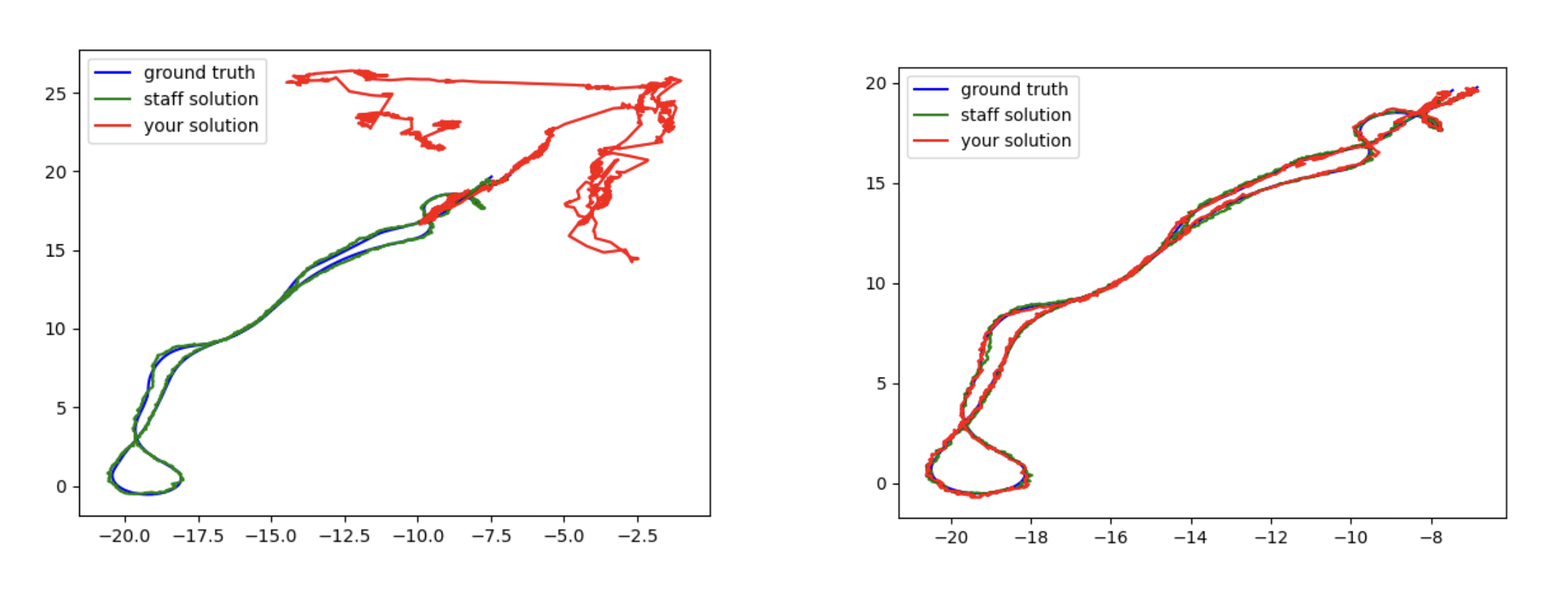
Figure 3.1.1 As seen above the untuned code on the left completely loses the car and its motion diverges. Lidar sensor updates are unable to save this. Tuned parameters on the right are accurately following the car, allowing us to receive 90%+ accuracy when compared to an expert solution.

Simulation Evaluation

[Carolina]

To evaluate our particle filter in simulation, we introduced noise in two places. First, we added an initial offset to the y-position of the particles in our cloud, and second, we added a normalized distribution of noise scaled by varying factors to each element of our odometry data (x, y and theta). The initial offsets were [0.2, 0.5 and 0.1] and the odometry noise scale factors were [0.5,0.5,0.2], [0.1,0.1,0.2] and [0.3,0.3,0.3]. For every pose estimate published, we logged the error (writing it to a CSV file), which was calculated as the actual position we estimated minus our expected position (which we could obtain from the transform).

To test our particle filter, we ran our wall follower algorithm from Lab 3 in RVIZ with a combination of an offset and odometry noise. Overall we recorded 9 trials of data. We separated our graphs into three levels for low, medium and high odometry noise. On each graph, we plotted the overall error in the x position vs time for each of the three offsets.

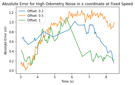
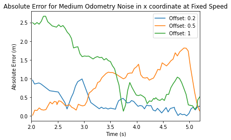
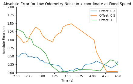
Figure 3.1.1, Figure 3.1.2, Figure 3.1.3 We can see across low, medium, and high odometry noise that our algorithm still performs well. The low and medium odometry noise graphs converge to 0 after around 5 seconds, and we see this pattern happening as well for the high odometry graph at 8 seconds.

Racecar Evaluation

[Ishita Goluguri]

Evaluating the particle filter using real data collected from the racecar posed a whole different set of challenges. To evaluate, five rosbags were collected: three from manually driving the car along the same stretch of hallway. Just as in simulation, the average x, y, and theta values were logged. From here, a new challenge arose- finding the ground truth odometry. While in simulation, it was possible to use the transformation between the map and base_link, in real life, it was difficult to find an alternative to strenuously measuring the ground truth odometry with a meterstick.

[Quinn Bowers]

To find the ending location of the robot in the map frame, we used visualization software to manually match the robot’s lidar data to the map. We presume this estimation to be roughly as accurate as using a meterstick to make manual observations.

[Ishita Goluguri]

Several graphs were created to analyze percentage error between the expected position and actual position of the three runs. Percentage was chosen over x,y, or theta offset because it seemed like a good metric to determine how far off the car was from the measured final value and how it converged to this value over time. This also allows a method of fair comparision across multiple trials. The three graphs generated below show the error of each measurement.

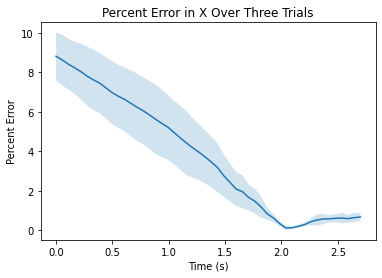
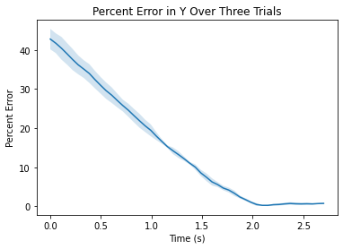
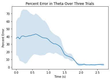
Figures 3.2.1, 3.2.2, 3.2.3. Showing percentage error between true position and predicted position in various directions as a function of time

In addition, the convergence rates in each of the three directions were plotted and averaged over the three trials. The convergence rates are fairly consistent amongst the three trials and the three directions.

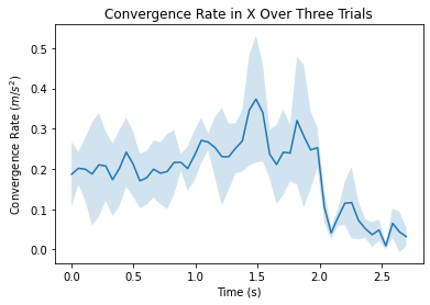
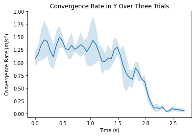
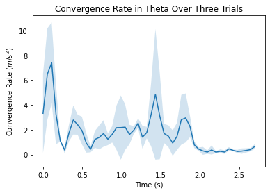
Figures 3.2.4, 3.2.5, 3.2.6 . Showing convergence rate between true position and predicted position in various directions as a function of time

Conclusion

[Vedang]

In this phase, we add complexity to the robot by providing a solution to the simple question: where am I? It is a skill that humans often take for granted, localization for a robot is a difficult task and an active area of research today. We solved this problem using a popular framework known as the Monte Carlo Localization (MCL) method or the Particle Filter. While this is just one algorithm in an expansive area of research, its complexity makes it challenging to implement but effective after rigorous tuning.

Unlike previous work done by the group, localization is not a control problem - it does not affect robot motion in any way. It utilizes the robot odometry and lidar data to update the orientation and position of small particles. These particles, with assigned probabilities, give a prediction of a possible location of the robot. Injected particle noise allows robust robot tracking over diverse velocities and environments. Added odometry noise ensures an accurate simulation to reality conversion. All these components moving in parallel allow us to locate our robot using a map and sensor data.

In the following lab, we are ready to build on the localization framework, with path planning. The combination of localization and path planning are the final two pieces needed to take on the final challenge - the culmination of all the work done so far. Having picked up essential debugging and coding skills so far, we plan to apply them in the path ahead.

Lessons Learned

Vedang L : Understanding the project early on and delegating tasks as needed was a key lesson I learned in this lab. Unfortunately, this was a lesson learned not through success but through failure to do so. While the presence of spring break decreased our progress, the intense, last-minute cram that followed after the break may be resolved with more disciplined work done earlier in the week. A key solution to this might be to ask TAs how long they expect each part of the lab to take. This should result in an even division of the work and minimize the chance of underestimating a task. The addition of a new teammate in the next lab may help with the division of work, increase day-to-day progress and decrease individual workload.

Through this lab, I gained a deeper understanding and practice of ROS. I finally feel confident in my ability to navigate the ROS architecture, syntax, and debug. Lastly, I learned the importance of finishing individual components earlier than the last day. Putting together different pieces of the lab almost always causes unknown issues to arise. Completing the lab done early and taking the help of a TA would reduce the time taken. With more time to submit and attend office hours for this next lab, I hope to make early progress on the lab. Through more discipline, we can only contribute to our success.

Ishita G: I felt that this lab was challenging both technically and in terms of organizational skills. It covered a lot of material, especially mathematical material, and it was difficult to understand at first. I felt that the problems assigned before the lab really helped figure out how to implement the motional model and the sensor model. In addition, the structure of this lab was unique in that everything relied upon previous parts and it was necessary to test each part meticulously before moving on to the next. This was helped greatly by the given unit tests, but there were still times where everyone was working on the same code. This introduced me to the concept of threading to ensure that people didn't work on the same code at the same time. In terms of organization, it was important to keep a checklist for this lab since there were many parts due. In previous labs, this wasn't as important. In addition, having spring break in the middle made it feel like we had less time than previous labs because of team members leaving early or getting back late. While we handled this well by making time during the week, in future labs, it would be good to do things as early as possible and have only a little work to do after a major break.

Carolina W: This lab was certainly a challenge and a learning experience for the team and especially for me. Part A of the lab was helpful for learning the background concepts and understanding the mathematical calculations behind the motion and sensor model. However, it was difficult to place these in a coding context. I fell behind on understanding parts of the code, since it was difficult to work in a way that allowed the whole team to understand every portion of the code we were writing. This made collaboration complicated later on in the lab, as we had to understand one another’s code to help with the debugging process. Using clear comments, and also taking opportunities to regularly check in with one another and ensure everyone is on the same page will help our team in the next lab. Not everyone needs to be an expert of every portion of the code – however, having a basic understanding of what each block of code does, what the inputs and outputs should look like, and how the pieces work together, is essential.

During this lab, I also learned a lot about best practices for evaluating algorithms and representing data. It was helpful to think about what information our graphs needed to convey to most effectively show that our algorithm worked well, and also how we could go about testing the algorithm in a controlled way. In the end, our team pursued a successful evaluation strategy, and I will carry this forward going into the next labs and final challenge.

Quinn B: The technical lessons I learned this week revolve mainly around interacting with roscore through less usual methods. Much of my debugging this week involved figuring out ros bags, and interfacing them with other ros systems in a way that doesn’t damage transform data. Beyond this, the lab went smoothly by and large, excluding a few gripes with the test cases. Another thing I learned this week was that local tests are for our benefit, and can be skipped if we know our algorithm is working. We spent many hours trying to figure out why our data didn’t match the test case data in a few very specific cases, and it turned out it was due to different indexing conventions and nothing that would have actually influenced the effectiveness of our robot. I was reminded again this week of the necessity of distributing tasks. I have a tendency to take on all the work I know how to do, which resulted in a significantly higher workload than is ideal. Next week I will take concrete steps to avoid this, by distributing tasks farther in advance and attempting to take on more of a supervisory role.

Presentation

Download Links

Briefing Slides: Download Slides

Download Report